Analyses in more depth
In this chapter we consider constructing analyses in more depth. We return to considering high demand on physical items, to reiterate our requirement — we want to have an idea of which physical items are currently in high demand. This may indicate that actions such as the procurement of additional physical copies, or of digital resources are required.
How might this high demand for items be measured? One solution is to consider, over a previous time interval, a year, a term, etc. which titles had a high number of physical item requests. This is an interesting historical measure. For example, we can construct an analysis that lists the number of physical item requests, possibly the number of loans, and bibliographic information in a given time period. The analysis can be ordered by the number of requests and then provides a little insight into which items experienced high demand over the specified interval.
There is also a provided measure in requests,
"Requests"."Request Measures (Average)"."Average Time to Available (Days)"
which measures, on average, how many days it took until a requested item was available for a patron. If this is high, it may indicate a high demand item. If a title only has a single physical copy with multiple holds then, on average, the time to availability is going to be long for a patron. They will have had to wait for requests in the queue ahead of them to be fulfilled. Again, this will be a useful historical measure. Like measuring the number of physical item requests this can, and should, be measured over a specific time period.
Another metric could be the number of loans a physical title is experiencing over a time period. So, high numbers of loans equates in a way to high demand. Further, a high loans per copy ratio could be another indicator of high demand.
Another approach might be to consider the number of active hold requests, the number of available copies and hence the ratio of holds per copy. A higher ratio indicates a higher current demand. As we are considering active requests we can view this as a timely measure of demand. In particular a ratio greater than 1 indicates there are more active requests than there are available copies. This could be monitored on a weekly or daily basis to provide a more up-to-date view of demand.
In Alma, hold requests of the type "Patron physical item requests" are placed against a physical title. This is reflected in the Requests subject area. Available copies data, how many actual items we have, is from the "Physical Items" subject area. So we need to combine the data from the two subject areas, if a ratio of requests per copy is going to be constructed.
For any of these metrics, or others that can be devised, their suitability as a measure of high demand on physical items is going to depend on institutional needs, policies and processes.
The available data
To construct our analysis we are going to need columns from both "Requests" and "Physical Items". To begin with we will take a look at the relevant data columns available using two analyses, one in "Physical Items" and one in "Requests". We will be filtering the data to ensure we have only rows that we are interested in. We can also filter for a limited number of particular test records. This allows us to investigate and understand, in detail, the data and processes involved. We will consider how to best combine the two subject area data columns for the purposes of the analysis.
So, the data columns we are interested in for our final analysis will be:
-
From the Bibliographic Details, available from both "Physical Items" and from "Requests" dimension, — MMS ID, Author and Title.
-
the historical measure of the number of requests over a defined period of time.
-
the number of requests on a title, filtered to have an active request status, and by having a request type of patron physical item requests.
-
the number of physical items that are in stock.
-
the historical measure of the number of loans over a defined time period.
-
the ratio of requests per copy calculated as the number of active requests divided by the number of copies.
-
the material type, we may wish to distinguish between, for example, "Books" and "Bound Issues".
-
the call number, we might want to identify subject areas that have more high demand requesting.
-
the system provided measure,
"Requests"."Request Measures (Average)"."Average Time to Available (Days)".
The analyses for this chapter can be found in the folder
"<Your institutions folders>/AAPL Training/indepth"
and can be used as a reference. Remember it’s better to further familiarize yourself with "Design Analytics" by constructing your own.
Exploratory analysis in "Requests"
Let’s start with a new analysis in "Requests". We will need the columns:
-
"Requests"."Request Measures"."# of requests"
-
"Requests"."Bibliographic Details"."MMS Id"
-
"Requests"."Bibliographic Details"."Author"
-
"Requests"."Bibliographic Details"."Title"
-
"Requests"."Request Type"."Request Type Description"
-
"Requests"."Request Status"."Request Status"
-
"Requests"."Material Type"."Material Type Description"
-
"Requests"."Bibliographic Details"."Material Type"
-
"Requests"."Physical Item Details"."Permanent Call Number"
-
"Requests"."Request Measures (Average)"."Average Time to Available (Days)"
as shown in Figure 1.

Note that "Material Type"."Material Type Description" from "Physical Items" and "Bibliographic Details"."Material Type" (available in both subject areas) are different data columns and are not necessarily both simply "Book" in this analysis. For example, you may be able to see, some that have a "Physical Items" material type of "Thesis" and "Book" from "Bibliographic Details". This will largely be down to local conventions regarding material types (Is this true? Are there other reasons for this?).
In terms of the final data columns we want to display in our analysis these are nearly all that we need. However, when working from the "Requests" subject area there is no data column available that lets us know the number of available copies. There is a dimension for "Physical Item Details", such as "Barcode", available in the "Requests" subject area but there are no measures for the number of copies that are available.
One might reasonably consider whether to use the "Barcode" descriptive field from the "Physical Item Details" dimension. It is a unique identifier so a form of "count(distinct(Barcode))" might be considered as a number of physical copies. But, remember we are looking at the "Requests" subject area so that number would include only copies on which a hold requests had already actually been placed. So, in many cases we would be under counting the number of physical copies. The calculation, "count(distinct(Barcode))", would only accurately reflect the number of copies if it were carried out in the "Physical Items" subject area.
There is also a "Num of Items" data column in the "Physical Item Details" The only values it appears to take have been 1 or 0, so it would seem that it is just a count of the physical items for the request. It appears to have no other function I can see.
You can load the analysis "requests_analysis_1" from the catalogue or, for further practice, construct your own using the same columns.
The video, Exploring the requests data, investigates the data rows returned by "requests_analysis_1", showing some techniques for data investigation, and adds some useful filters. We need to filter for active requests and for those with the type being patron physical item requests. For simplicity, we will only be considering items with the book or issue material types. An analysis configured with these filters is saved in "requests_analysis_2".
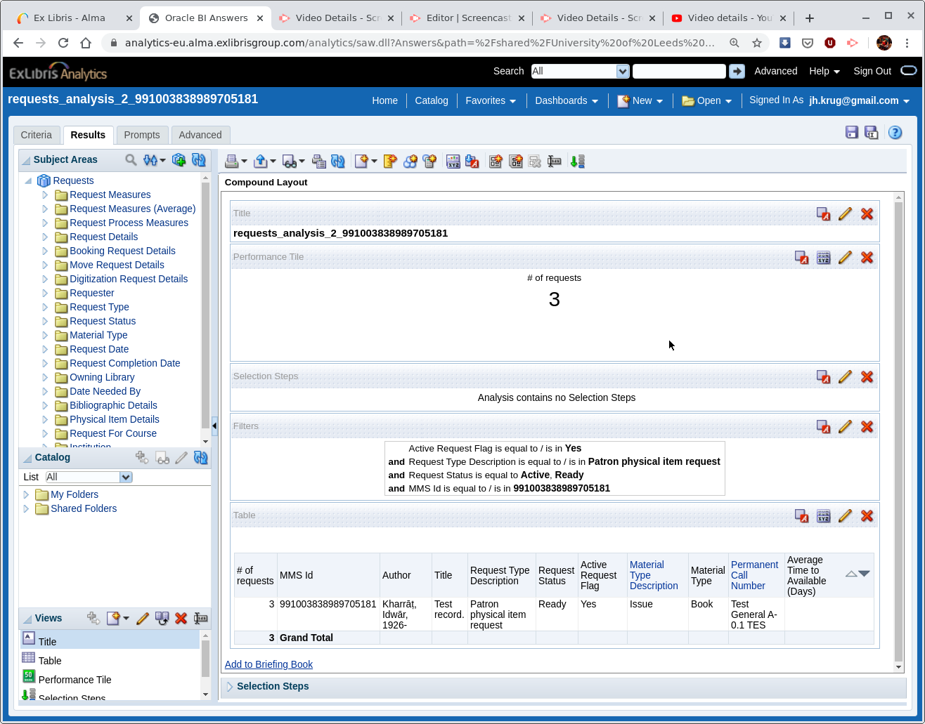
There is also an analysis "requests_analysis_2_991003838989705181", identical to "requests_analysis_2" but further restricted to a specific test record with the MMS Id "991003838989705181". We can use this to investigate more closely specific data for requests on a specific physical item.
| In this section, where we quote particular numbers such as there being 5 requests that we can see, we are relying on a particular set-up of test data, such as for the MMS Id "991003838989705181". This will change over time, and you will need to construct your own example using a MMS Id from your own data. The screenshots in Figure 2, Figure 3, and Figure 4 were taken prior to the interface upgrade in 2020, so look slightly different to now. |
The screenshot Figure 2 shows the results screen for the analysis "requests_analysis_2_991003838989705181".
Exploratory analysis in "Physical Items"
Now lets look at the available data from the "Physical Items" subject area. The relevant columns would be:
-
"Physical Item Details"."Num of Items (In Repository)"
-
"Physical Item Details"."Material Type"
-
"Bibliographic Details"."MMS Id"
-
"Bibliographic Details"."Author"
-
"Bibliographic Details"."Title"
-
"Physical Item Details"."Num of Requests (Physical Item)"
-
"Holding Details"."Permanent Call Number"
At first look it may appear that
"Physical Item Details"."Num of Requests (Physical Item)"
would be a good candidate for looking at the number of requests we need to calculate the active ratio of requests per copy. But this number is the total historical number of requests there have been on the item. It does not reflect the number of active requests as there are no details pertaining to request status available directly from the "Physical Items" subject area. That can only come from the "Requests" subject area.
Combining the required data columns
We know we have methods for combining subject areas into a single analysis from the "Understanding data" chapter. How could we use these?
Creating an analysis based on the results of another analysis
We could create an analysis in "Requests" which contains the MMS Id identifiers for active physical item requests on books and issues along with the number of requests per MMS Id. We can use this analysis to create another analysis based on it in "Physical Items". This analysis would correctly list the physical items on which there are hold requests.
But, what about the number of hold requests, from the "Requests" subject area that we need to calculate the ratio. The number of hold requests is still not available as the "filtering based on the results of another analysis" mechanism only allows the use of one column, as a filter, the MMS Id. It is not actually including the MMS Id from the base analysis, only matching on it. What we do have available in the "Physical Items" subject area is the "Num of Requests (Physical Item)" and as we have seen it is a useful historical measure but not a measure of the number of active requests.
Using set operations
Set operations in OAS (Oracle Analytics Server) are for the union, intersection or subtraction of one set from another. The sets must contain the same data types. What we are trying to do is include different columns from different subject areas which may or may not have the same data types. So, set operations are not suitable in this context.
Using combined subject areas
We have the mechanism for this. Remember that an analysis in two, or more, subject areas can contain measures from either subject area and that the descriptive data columns must come from shared dimensions.
This is straightforward to set up initially, so let’s do that by returning to an analysis from the "Physical Items" subject area we have already looked at "physical_items_1". To reduce the number of rows returned by the analysis, saving a bit of time, we have a filter on "Physical Items"."Physical Item Details"."Num of Requests (Physical Items)" saying that this measure must be greater than 0. That is to say there must have been at least 1 physical item request at some point past.
It is worth thinking a little about the appropriateness of this filter for the final version of the analysis that we are looking to develop. Do we wish to leave the filter in place when the number of rows have been reduced by other filter mechanisms that we will have used? We are not sure, based on the available documentation, whether this number is incremented as soon as there is a physical item request, when it has been accepted, or when it has been fulfilled. This is one of those situations where some help, or detailed knowledge of underlying data models, from Ex Libris may be required. If the measure is incremented only when fulfilled, and we leave that particular filter in place, then there is the danger that our analysis will miss currently active requests if there has been no previous requests at all on a particular item.
Considering "physical_items_1", this analysis has all the needed columns except for the number of patron physical item hold requests that are currently active. We can add the "Requests" subject area into the analysis and add the column for "Requests"."Request Measures"."# of requests". We could also restrict the MMS Id to "991003838989705181", the Leeds test data by adding a filter on MMS Id. You can load a copy of this to investigate.
Now taking a look at the results tab we can see that the number of requests "Num of Requests (Physical Items)" is 5. What does that mean? We can see from the requests' data analysis, restricted to "991003838989705181", that we ran previously, that there are 6 requests for that test record, 3 of which are active. Why the discrepancy? A detail of local processing? A question for Ex Libris perhaps? Pressing on, we have seen from the request data for this MMS Id that there are 3 active requests of the "Patron physical item request type". This is the number that we want in our physical items analysis, so we can use it to calculate the ratio of requests per copy.
How can we get just the number of active requests of the correct request type into this analysis? We can try to add a filter on "Requests"."Request Type"."Requests Type Description" and "Requests"."Request Status"."Request Status". But this will return no, or some data, but with some columns empty. This is because we are trying to include columns, or filter on them, in the analysis that are not from the measures or the shared dimensions. Remember that we can only use columns in a shared subject area analysis that are from the measures or are from the shared dimensions.
So, what we actually need is to filter the measure in the column "Requests"."Request Measures"."# of requests" to count only those which are active and of the correct type. Imagine this filtering is taking place on that column, from the "Requests" subject area, using filter columns entirely from "Requests". That is to say the filtering is not taking place in the joint subject area analysis, but only in "Requests" before it is used in the joint subject area analysis.
We can do this by editing the formula for the "# of requests" creating a custom measure that meets our requirements.
Go to the criteria tab and for the column menu for "# of requests" from the "Requests" subject area select the "Edit formula" option. Then select "Filter…". Now the screen should look as in Figure 3.
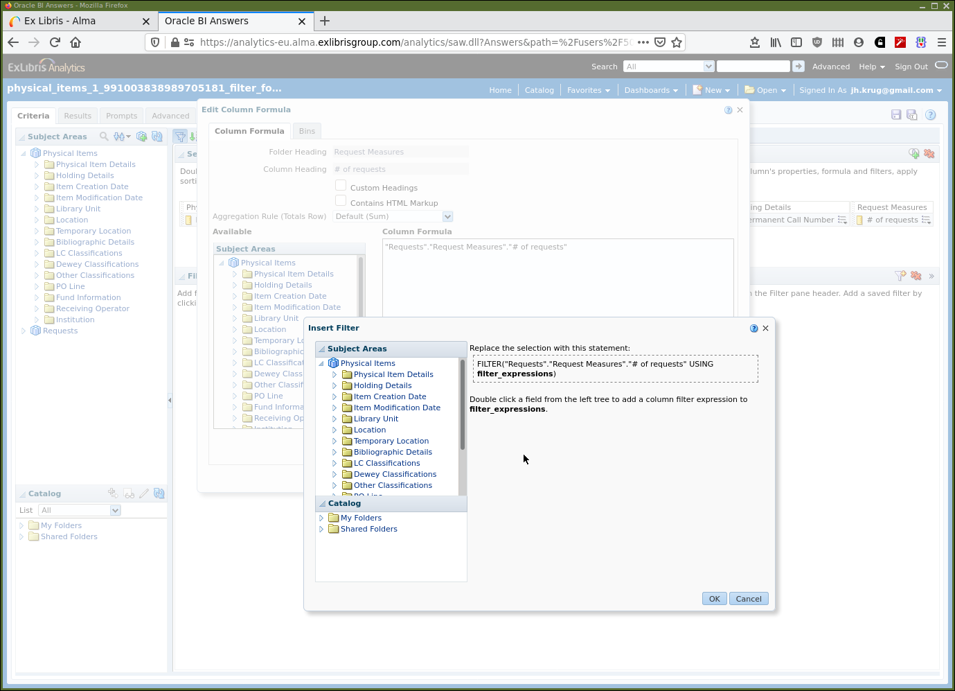
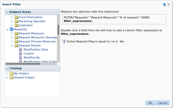
Using the "Subject areas" panel find the "Active request flag" in "Request Details", double-click on it to add it as a filter for "# of requests". We will now have the usual filter dialogue box that will allow us to say that the request flag should be set to yes. Do this to have the screen dialogue look as in Figure 4.
Click "OK" and the column formula box will now contain the code:
FILTER("Requests"."Request Measures"."# of requests"
    USING ("Requests"."Request Details"."Active Request Flag" = 'Yes'))
Now taking a look at the results table shows that the "# of requests" column, with the filter, now has the value 3 for this particular physical item. We also want this "# number of requests" to be filtered to only be counting requests of the type "Patron physical item request".
We could go through the process again, navigating the menus and dialogues to create a filter of a filter and that will work fine. It’s also equivalent to delete the filter already there, reverting to just the measure, "# of requests" and repeat the process to replace the "filter expression" with a new filter that has two filters in the filter expression, one on the active request flag being yes and the other of the request type being a patron physical item request.
In many cases, however, it’s easy and simpler to edit the filter formula directly. As follows:
FILTER("Requests"."Request Measures"."# of requests"
    USING (
        "Requests"."Request Details"."Active Request Flag" = 'Yes'
    AND
        "Requests"."Request Type"."Request Type Description"
            = 'Patron physical item request'
    )
)
Edit the column formula again to reflect the additional filter. A cut and paste of the above code should work fine. While we are there, before clicking OK we can fix the now ungainly column heading by selecting "Custom Headings" and replacing the text in the "Column Heading" text box with "Active PI requests".
We can now create our ratio calculation column. There is no direct way to create a column from scratch, but we can select any old column from the subject area panel and replace its definition, including its headings, with what we require. We need to edit the column formula to be Requests/Copies. We need to change the column heading, again, to make it less ungainly. We will also need to change the default data format, using the column properties dialogue so that the ratio has a couple of decimal places.
So, to make all that clear, lets try using the analysis "physical_items_1" as the base for constructing this, as shown in the video High demand on physical items.
Adding further functionality
Variables
It’s possible, to some extent, to define and use variables within the Ex Libris implementation of OAS. For example, we might wish to prompt for a date range, and store the start date and the end date in variables. Then we can use those variables to display the date range as part of the analysis format or to use within filters in the analysis.
The variables we are interested in using are referred to as "Presentation Variables" within OAS. There is more information[mwug] available in Oracle’s documentation. There are other types of variable, but they do not appear to be generally available in the Ex Libris implementation, e.g. system variables and system presentation variables. It’s best to rely only on presentation variables that we ourselves create.
Working with dates & time
All analytics is going to be concerned with date & time as a context, often it is the primary one for any analysis. Data concerned with loans, requests, orders, courses, etc. is usually going to come with an implicit, question, "When is this data applicable?"
So, here are some date related tasks that we will wish to know how to do:
-
How can we filter for a particular date, filter for data greater than, or less than, or between dates?
-
How can we ask the user of an analysis what date range they are interested in and when they have answered how do we store and use that date range?
-
How can we supply defaults for date ranges, for example to pre-populate a prompt?
-
How can we compute the difference between two dates? For example, the difference between the loan date and the return date.
-
How can we add a constant to a date? For example, what is the date in "today + 30 days", or in 12 weeks?
You will have noticed while looking at column formulas that there are "Calendar/Date" functions that can be applied to our data columns where they contain data corresponding to dates, time and timestamps. A timestamp is a date and time combination, e.g. "2007-04-01 19:45:25". We shall take a look at some of these functions and some basic usage.
A variable in OAS is referenced (or used) using the following syntax:
"@{variable_name}{default value}"The default value part is optional but very useful. If you can imagine a computer program talking its way through a computation in English then the line above says …. "Give me the value for "variable_name" if set, if it has not been set then give me the value for "default value" instead".
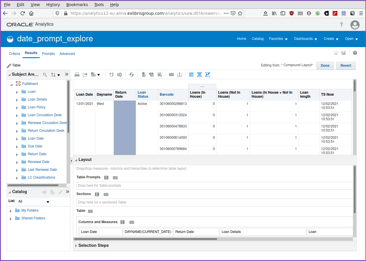
Let’s work through an example using variables and dates. Find and load the analysis "date_prompt_explore" in the "AAPL Training/indepth" folder. There is quite a bit going on in this analysis so let’s investigate in the video Date functions and prompts.
Adding totals and sub-totals.
It’s often useful to be able to see aggregate numbers of events. Returning
to the analysis "date_prompt_explore", how can we add a sub-total of loan
numbers by days and a grand total of loan numbers? We need to format the
container containing the table body of the analysis. Clicking on the edit
pencil icon,  , for
the "Table" panel, while in the results tab will bring up the screen shown in
Figure 5.
, for
the "Table" panel, while in the results tab will bring up the screen shown in
Figure 5.
We are looking to apply totals for the "Columns and Measures" section. Look for
the summation symbol,  , in "Columns and Measures". As examples, click on the summation symbol
for all the "Columns and Measures" and also for the specific column, "Day
Name". In both cases select "After" from the menu. The screen will update in
the preview panel and totals will be generated for each "Day Name" as well as a
"Grand Total". When finished modifying the layout, or experimenting with it, be
sure to click Done, or Revert for the table layout editor.
, in "Columns and Measures". As examples, click on the summation symbol
for all the "Columns and Measures" and also for the specific column, "Day
Name". In both cases select "After" from the menu. The screen will update in
the preview panel and totals will be generated for each "Day Name" as well as a
"Grand Total". When finished modifying the layout, or experimenting with it, be
sure to click Done, or Revert for the table layout editor.
The video in Adding in totals and sub-totals shows this in action.
Adding date ranges, prompt and totals into our high demand reporting
Now we can return to our high demand analysis, saved as "high_demand_reporting". Prompts have been added to restrict the date range to which the analysis applies and totals have been added. The video Dates prompts and totals in high demand reporting shows these additions.
Some other useful techniques or technical details
Adding a visualization or pivot table
OAS provides a wide range of graphs that can be added to an analysis. It will also attempt to suggest the best visualization depending on some sort of heuristics it must be applying to our analyses and data.
A visualization can be effective at communicating information, particularly trends over time. A visualization is of no use if the meaning of the data is not well understood and can be misleading.
Wikipedia expresses the concept of the pivot table well. It’s a table providing a summary view of the available data. You can think of all visualizations, whether a pivot table or graphical, as attempting to aid understanding by summarizing and simplifying a large data set to better show features or trends and to possibly make predictions.
| From Wikipedia[wppt] — A pivot table is a table of statistics that summarizes the data of a more extensive table (such as from a database, spreadsheet, or business intelligence program). This summary might include sums, averages, or other statistics, which the pivot table groups together in a meaningful way. |
In OAS a pivot table is regarded as being one of the available visualizations. If, using our high demand analysis as it currently exists you ask OAS to insert the recommended visualization it will use a pivot table. Which is sensible if you consider the content of the analysis so far, we are concentrating on finding items that match a particular requirement, that they are in high demand. It is not time series data. In this analysis we are not looking at a trend over time when a graphical visualization becomes more appropriate.
We shall look further into the available visualizations in the chapter on format and style.
Briefly here, in Adding a visualization, we look at adding some visualization so that you can start exploring and trying them out in your development and exploration.
Bins, or buckets, or containers
Bins, or buckets are a mechanism for collecting together data items which share characteristics into a kind of container. They are collected together into bins, in the OAS parlance. We can illustrate how we might use bins in the context of a custom classification scheme. By custom, we mean a classification scheme that is not Library of Congress or Dewey . There is plenty of support in AAPL for the standard schemes. Your institution may do something different. For example, University of Lancaster uses BLISS and University of Leeds has a full custom classification scheme.
A custom classification scheme uses the "Permanent Call Number" data column as in "Physical Items"."Holding Details"."Permanent Call Number". Consider the screenshot Figure 6 from the University of Leeds. It shows an analysis showing the number of items associated with each distinct call number.
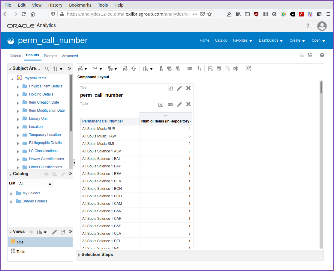
Consider the call numbers "All Souls Music BUR", "All Souls Music HAW", and "All Souls Music SMI". "BUR", "HAW", and "SMI" probably refer to the Author. For the purposes of the analysis we might wish to group them together into a home-made classification top level of "All Souls Music".
Let’s try this using bins. Follow along in the video Introduction to bins.
You can see that this can get complicated fairly quickly. Note that we have the "Save Column As" option which allows us to save our column bins formula definition as a reusable component. We can then reference it in a different analysis, also in the "Physical Items" subject area. We can see from the column definition that defining some bins generates SQL that the analysis uses. This opens up the option, useful along with "Save Column As" of keeping the SQL code outside OAS in a source code control environment and where the code can more easily edited, using your preferred text editor, than within OAS.
Code similar to that shown below could be created in text editor and then pasted into the "edit formula" definition panel in OAS. The column definition can then be saved and reused.
CASE
    WHEN
        "Holding Details"."Permanent Call Number"
    LIKE
        'All Souls Music%'
    THEN
        'All Souls Music'
    WHEN
        "Holding Details"."Permanent Call Number"
    LIKE
        'All Souls Socinianism%'
    THEN
        'All Souls Socinianism'
    WHEN
        "Holding Details"."Permanent Call Number"
    LIKE
        'All Souls Science Periodicals%'
    THEN
        'All Souls Science Periodicals'
    WHEN
        "Holding Details"."Permanent Call Number"
    LIKE
        'All Souls Science%'
    THEN
        'All Souls Science'
    WHEN
        "Holding Details"."Permanent Call Number"
    LIKE
        'All Souls Theology%'
    THEN
        'All Souls Theology'
ELSE
    "Holding Details"."Permanent Call Number"
END
If there is a need for reporting against top line classification (or other local grouping requirements) it may be worth developing this concept further at your institution. Of course, bins are useful in many other areas as well.
Adding interactivity
When using an OAS analysis, we might like to have some element of interactivity. Perhaps we could click on a column heading to invoke an analysis in a different subject area using data from the analysis we are currently looking at. We might want to select a data item in a column and invoke an analysis that provides further information on that data object, or to link to that object in the online catalogue. We can add column interactions from the "Criteria" tab and editing "" to add "Action Links". "Action Links" are the mechanism whereby an action is specified for when a link defined for a column is clicked.
The video Adding interactions, using the analysis "high_demand_reporting_with_vis" shows an introduction to how this can work.
Note that the Primo search and the fulfilment history interactions may not necessarily work on your selected data items. For Primo, that item might be suppressed from a catalogue search and for the fulfilment history action there may be no fulfilment history to display.
KPIs and watch-lists
| KPIs and watch lists do not appear to be supported in this instance of Oracle Analytics (since October 2020). This section is left as a reference and only applies to the previous releases. This may well change. |
Key Performance Indicators (KPIs) are described in the OAS Users Guide[mwug] as:
"KPIs are measurements that define and track specific business goals and objectives that often roll up into larger organizational strategies that require monitoring, improvement, and evaluation. KPIs have measurable values that usually vary with time, have targets to determine a score and performance status, include dimensions to allow for more specific analysis, and can be compared over time for trending purposes and to identify performance patterns."
So, a library goal might be that there should be no more than "n" patron physical item requests being made per day. Or, no more than a "p%" increase on the previous day. Possible reasoning might be that, if there is such a number of requests being made or such an increase then it needs to be noted. Perhaps to devote effort to making sure adequate copies are available or to steer requests towards available digital resources.
Given this information we can create a KPI to measure this. This KPI would then be able to be used within dashboards that we create. In the video Creating and using a KPI and watch-list we shall consider some, somewhat arbitrary KPIs, incorporate them into a KPI watch-list, a collection of KPIs, and then use it in a dashboard.
Analyses in more depth — final points
We have seen that it can be fairly easy to misinterpret the data that is presented to us. It’s worth paying attention to the detail of the questions we are asking, how the data is represented in Alma/Primo/Leganto and within OAS, and the results of our analyses. It is the author(s) views that Analytics work is not only a technical endeavour. It’s vital to have an experienced librarian eye on the questions, the details of analysis implementation and the source and result data and the processes that generate them. Of course, this librarian can also be the same person as the analytics technician.
We should also remain aware that it’s worth thinking of the subject areas as providing answers to a set of class of questions that have been framed by the Ex Libris implementation team. They have codified their implementation in the OAS data model and the ETL to produce the subject areas and their contents. OAS is not a general purpose query tool. We have seen it’s possible to answer some questions that have not been fully catered for by the OAS data model by constructing analyses that combine two or more subject areas.
If we need additional functionality or data to be available from the data models then Ex Libris will need to be approached. This could happen via the SIWG and/or the enhancements process, to make adjustments to the data model and ETL.
So, it is reasonable to say that if a valuable query requirement is rather difficult to implement in Alma, Primo or Leganto Design Analytics, possibly even impossible, then it is also worthwhile to consider if the OAS analytics data model and the ETL need some modification by Ex Libris.
Effective analytics is as much about deep experience of the processes that generate the data and the data itself as it is about the tools, i.e. OAS, available for manipulating that data.
Exercises
-
Take your own copies of "requests_analysis_1" (or make your own) and "requests_analysis_2", store them in your "My Folders" area and investigate and experiment. Add the filters to "requests_analysis_1" to create your own "request_analysis_2"
-
Adjust the filter expression for the "# of requests" measure column. Add a filter to the filter expression that additionally restricts the data to only those requests which are on a material type of book or issue.
-
Create an analysis (there is a solution in "date_answer"), it is possible to use any subject area, that returns a single line with the following columns:
-
the current date
-
the day of the month number of the current date, e.g. for 2021-01-03 return "03"
-
the year component of the current date
-
the date in 12 weeks time from the current date
-