Understanding your Analytics data

The aim of this chapter is to provide sufficient information regarding the sort of data available to analytics to enable you to work with it. It aims to give you an idea of the origin of the data, how it is arranged, and what type of operations can be done with it. It’s not intended to be a comprehensive set of documentation regarding the subject area and the available data fields within them. That is provided by the Ex Libris documentation available from their Knowledge Centre.

The data that you look at when doing "Design Analytics" is data that that has come from your Alma instance at your Ex Libris regional data centre. The data you are looking at is in the OAS data warehouse, a different type of database to the Alma instance, and to be clear, still at an Ex Libris data centre.

Consider the dates marked out in Figure 1. "Data updated as of" is the timestamp when the extraction of data from your Alma instance started. "Data available as of" is when that data was available to look at within AAPL.

Generally this extract will be scheduled and finished overnight at your regional data centre, but the process does occasionally go wrong or have delays. You can see that the data extract shown in Figure 1 took approximately 5½ hours.

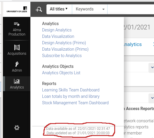
Figure 1. Analytics data extract date

The important date is the "updated as of", data generated in Alma after that date will not yet be visible within analytics.

It’s necessary to keep in mind that the data in Analytics is not the same as that in Alma, or Primo, or Leganto. The data is extracted from Alma, Primo or Leganto (APL), which are data transaction processing systems. The data is then transformed into a form suitable for the warehouse data model, designed for business analytics and reporting, and loaded into OAS. This process is commonly referred to as Extract, Transform and Load (ETL) in the data processing business. You may also see references to ELT (extract, load, transform) which is a slightly differing method of achieving the same result. Wikipedia has more information[wpdw].

The ETL is a multiple component hardware and software process and these complex processes may have bugs.

Why do this, why not just construct analyses from the APL data directly? The reason is that Alma, a transaction processing system, is optimized for processing large numbers of operations on smaller chunks of data.

In contrast, OAS, designed for reporting and data analysis, is optimized to perform complex queries on large numbers of those chunks of data.

In a system that attempted to merge these two paradigms we would be trying to scan large amounts of data, to do analytics, whilst at the same time trying to do transaction processing, all of which would be using the same processing and data storage hardware, software, and other infrastructure. All of which would be optimized for neither use case. It would be a recipe for data traffic jams, of data transactions and data searches.

Why is understanding this distinction important? We are trying to develop analyses that give us insight into our library operations. We need to have understanding of the source and history of the data we are looking at. As librarians looking at our data in AAPL it’s not, in general, possible to have a complete understanding as the Alma and OAS data models and the transform process are proprietary. In normal use this is will not be an issue, but if we find ourselves occasionally puzzled by the data we see in Analytics then it may be worth remembering this. It is derived from the data in APL but is not the same as the data in APL.

It’s also the case that while AAPL contains a vast quantity of useful data extracted from Alma, Primo or Leganto it will not contain all the APL data. The construction of the ETL or ELT entailed making decisions regarding which data fields to extract and which to not. This is normal and expected, APL and OAS are different systems with different purposes. Additionally, there will be computed data in OAS which is not available in Alma. For example, the "# of requests" data fact/measure that we have been using in our analysis may not exist in Alma. It could be that that measure value is computed during the transform part of ETL and stored only within OAS.

If puzzlement does occasionally arise then Ex Libris are able to help via their standard support mechanisms. IGeLU and ELUNA are also involved in product enhancement requests, which may be necessary.

Subject areas

Now we have the necessary discussion of the nature and genesis of analytics data out of the way we can consider subject areas and there relationships to each other in more depth. Ex Libris maintain a document, the Alma Product Documentation for Analytics[aag], which is updated with each release of Alma. It provides documentation for the available data subject areas and the data fields. There is also the Primo Product Documentation for Analytics[pag]. At the time of writing (2025-12-11), the documentation for Leganto analytics is with the Alma documentation, as the Leganto subject areas are included with the Alma subject areas.

A star schema is a means of representing a set of one or more fact tables and any number of dimension tables. It is commonly used to give a visual representation of a data warehouse data model, or subject areas.

We constructed our first analysis on the "Requests" subject area, so how would the data we used for that analysis look as a star schema diagram. Consider Figure 2. The fact table, "Request Measures", from which we are selecting "# of requests" sits at the centre. The dimensions, radiating from the centre, contain descriptive information relating to the facts.

Figure 2. Requests Subject Area — simplified star schema

Looking at this simplified star schema we can think about our "physical items in demand" analysis as follows:

We are interested in a library fact, the number of requests we have on physical items.
For our current purpose we are only interested in those where the request status is active and where the request type is "Physical Item Request". We did this by using filters, not shown in a star schema.
We are interested in knowing the MMSID, Author and title for these current requests.
Not shown in the schema but used in our analysis, we used a prompt to only get information on items where the number of requests was greater that a number provide by the user at runtime.

The star schema is a method of documentation of the data within AAPL and simplified versions, as we have constructed, could be used in documenting your own analytics developments. You will see star schemas used in Ex Libris documentation on analytics.

Note that the representation, in a hierarchical style, within the analytics editor is more or less equivalent to a star schema. The measures are at the top rather than in the centre and the descriptive dimensions are hierarchically listed rather than being arranged around the facts table.

Any analysis should contain at least one fact or measure. An analysis that contains only descriptive information is likely to run slowly, and may time out.

Multiple subject area analyses and shared dimensions

Most analytics queries will have no need to use more than one of the available subject areas, but, occasionally, some will.

Ex Libris have constructed the AAPL OAS data model defining the subject areas for use in our analytics efforts. The subject areas are based on what Ex Libris and development customer partners decided that libraries will need to be reporting on. In most cases these subject areas will be adequate for our reporting needs. A subject area, then, will exist and have been designed to be capable of answering a set of common or likely reporting tasks within that subject area. It aggregates data from different parts of the Alma data model in order to answer those business analytics queries.

Shared dimensions

A shared dimension is a dimension that appears in more than one subject area. For example, "Bibliographic Details" is a dimension that is present in both of "e-Inventory" and "Physical Items". It is also in many other subject areas. It is present in both as it’s useful dimensional data for queries in both of those subject areas.

Multiple subject area analyses

It might be necessary to develop an analysis that bridges more than one subject area in order to meet your particular needs. This will be because a subject area does not exist that contains all the fact data fields that are needed. It is worth reiterating that this will not usually be necessary as the subject areas have good definitions and contain a comprehensive selection of fact and dimension data fields.

In order that such an analysis will succeed, there are some conditions that must be met. These are:

The subject areas in the analysis must have a dimension in common, i.e. a shared dimension such as "Bibliographic Details"
The descriptive fields used in the analysis must come from the shared dimensions.
The measures used can come from any of the subject areas in the subject areas. As many measures as required from any of the subject areas included can be used.

Let’s work through this by considering an analysis using "e-Inventory" and "Physical Items". We want an analysis that shows us both the number of eInventory portfolios and the number of physical items that we have. It will contain the columns for "e-Inventory.Portfolio.No. of Portfolio (In Repository)" and "Physical Items.Physical Item Details.Num of Items (In Repository)". We also want the result broken down by "Library Name" and whether the items are suppressed from discovery.

The video, An analysis using two subject areas, shows how this might be constructed, how to add additional measures from either subject area and what happens when descriptive dimensions are chosen that are not from the shared dimensions. It is worth noting that the shared dimensions may not have exactly the same name in both subject areas. "Bibliographic Details" is named the same in both subject areas but "Library Name" comes from "Portfolio Library Unit" in "e-Inventory" and from "Library Unit" in "Physical Items". It can make finding them a little difficult sometimes.

An analysis using two subject areas

A completed version of the analysis used to illustrate multiple subject areas is in "/shared/University of Leeds 44LEE_INST/AAPL Training/data" and the analysis is called "eInv_pItm".

Analysis based on the results of a different analysis

Another mechanism for using data from more than one subject area is to use the output from an analysis in one subject areas as an input for filtering an analysis in a different subject area.

Let’s consider another example. In the "Design Analytics" editor locate the analysis called "fines_gt_50" in the shared folder "/shared/University of Leeds 44LEE_INST/AAPL Training/data". Select the criteria tab, so the screen should look like that seen in Figure 3.

Figure 3. Fines ≥ 50

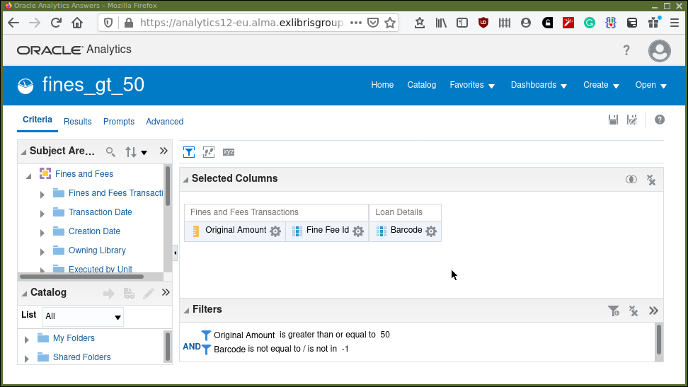
What we have in Figure 3 is an analysis that produces three columns, the original amount of the transaction, barcode, and the fine-fee id it was associated with. We have filtered the analysis, so we exclude a barcode of -1. The "-1", probably represents fines and fees on things for which there is no associated barcode. We also filter by the amount, we are looking for item barcodes generating fines/fees greater than 50.

Consider the result in Figure 4.

Figure 4. Fines ≥ 50 result

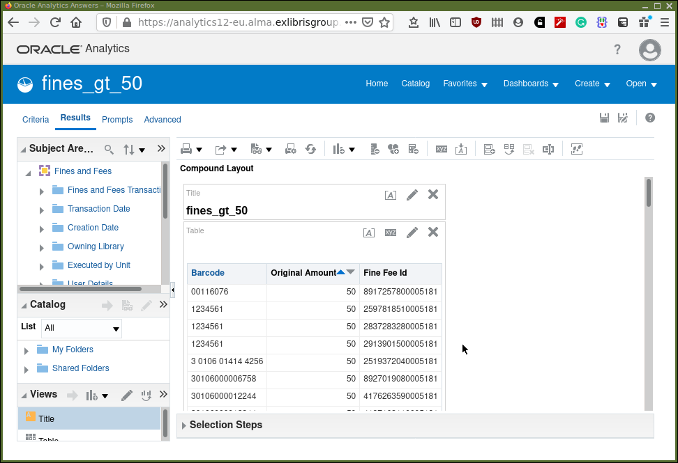
We can see for example (at the time the analysis was run and the screenshot taken) that for the barcode "1234561" there have been three fine/fee transactions where the original amount was 50.

Imagine that, for some strange reason, we want to know the item creation dates for those barcodes which have generated transactions greater than 50. There is plenty of information available from the fines and fees subject area but not the item creation date.

In the same folder is an analysis called "item_creation_date_using_fines_gt_50". Open it and navigate to the Criteria tab. You will see that the selected columns are "Barcode" and "Item Creation Date". Note the filter panel. That filter says to select barcodes which match, are equal to, those barcodes in the analysis "fines_gt_50".

What happens when executing the analysis "item_creation_date_using_fines_gt_50" is that, first, the "fines_gt_50 analysis" is executed, and it’s results then used as input to complete the item creation date analysis.

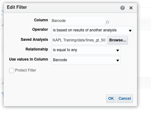
With the mouse, highlight the filter and click the edit pencil icon, so we can take a closer look at the filter definition in Figure 5. We are filtering, in this analysis, on the barcode column. The filter is based on the results of another analysis, which is defined in the "Saved Analysis" field. The relationship is equality and the values from the barcode column in the included analysis should be used for the match. Click around on the drop down menus to see what other options are available.

Figure 5. Filter definition for the item creation date analysis

Close the definition panel and select the results tab to see the list of barcodes and associated item creation dates. The barcodes being those from the first analysis which filtered barcodes with high fine/fee levels.

Using set operations to combine subject areas.

This too is possible but is potentially hard to think of within the complexity of library data. Set operations are logical operators which combine two sets of results, either two queries in the same subject area or two queries in different subject areas. It is important to note that a set operation can only be carried out on two sets that have the same columns. So, it is not so much a combining of data from two subject areas as performing logical operations on results, of the same type or containing the same types of data, from two areas. So, for, example you could look at "e-Inventory" items and "Physical Items" and consider bibliographic records that are in both subject areas. The set operation could tell you which bibliographic records are in both (intersection), just one (minus) or either (union) of the result sets. "Union all" is the same as union but includes duplicates.

Our example will consider titles in "e-Inventory" and "Physical Items" by Orwell and combine the results using set operations to determine:

All the titles we have by Orwell, in either "e-Inventory" and in "Physical Items" (union)
All the titles we have by Orwell, in both of "e-Inventory" and in "Physical Items" (intersection)
All the titles we have by Orwell, in just one of "e-Inventory" or in "Physical Items" (minus)

The video shows an example of working with sets.

A analysis using set operations in two subject areas

If you want to look at the analyses used they are located in "/shared/University of Leeds 44LEE_INST/AAPL Training" and are called "set_1", "set_2" and "set_1_and_2".

Understanding your Analytics data — final points

AAPL data is derived from APL data via an ETL process. Software and hardware, and design decisions, possibly involving competing priorities, are involved in populating your analytics database.
Multi subject area reporting is difficult to understand and to implement. Reporting requiring this should rarely be necessary as the defined subject areas are well implemented with comprehensive measures and descriptive fields. (It’s fair to say that this is mostly true, however it will always be the case that specific requirements will need multi subject area reporting.)

Exercises

Take a copy of "eInv_pItm" to your private "My Folders". Experiment with including different measures, shared dimensions fields, and non-shared dimension fields.
Redo the set analysis but with "Physical Items" first, then bring in "e-Inventory". This will allow you to see the effect of the minus set operation with the larger set first. Take a copy of "set_2" to your private "My Folders" as a basis to start work with.

Unfortunately there does not appear to be a way within the analytics editor of rearranging the order of the subject areas to achieve the same thing by editing "set_1_and_2" directly.
The examples of multi subject area analyses seem contrived. Can you think of more realistic scenarios from experiences at your own institution? Please let the author(s) know, they would like to incorporate further examples that are more plausible and hence relevant.